Part 10: Surviving the Real World — Fault Tolerance, Self-Identification, and Security
Welcome to the finale of "Robotics Zero to Hero." Parts 1–9 built a robot that can think: it knows its geometry (Part 1), its kinematics and dynamics (Parts 2–4), it can plan (Part 7) and reason with learned models (Parts 8–9). Part 5 confronted the sim-to-real gap — the moment theory meets a noisy, frictional world.
This post is about what happens after deployment, when the robot is alone in the field and things start to break. A tendon snaps mid-task. A sensor begins to drift. The payload is heavier than the model assumed. An adversary injects false data onto the bus. A deployable robot is not the one that performs best in the lab; it is the one that notices something is wrong, figures out what changed, reorganizes the actuators it has left, re-identifies its own physics, learns the new task it is handed, and does all of this while under attack.
These capabilities form a single feedback loop, drawn below. The rest of the post walks around it.
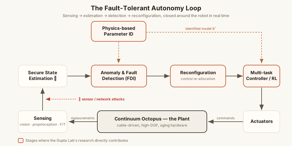
Figure 1 — The fault-tolerant autonomy loop. Highlighted stages are where research from the Gupta Lab at Ohio State directly contributes; we flag each contribution in a Research Spotlight block.
How to read this post. Throughout, blocks like the one you are reading collect the specific research contributions that make each stage work, with links to the papers. They are the load-bearing walls of the loop in Figure 1 — read them to see why each piece is hard and what was actually proven.
1. Anomaly Detection: Noticing That Something Is Wrong
The first line of defense is a detector that turns a stream of sensor data into a single binary question: is the robot still behaving normally? The workhorse is the residual — the gap between what a sensor reports and what the model predicts:
In a healthy robot is zero-mean noise. A fault, a collision, or an attack shifts its statistics. The classical detector is CUSUM (cumulative sum), which accumulates evidence of a mean shift and alarms when the evidence crosses a threshold :
The trade-off is eternal: lower detects faults faster but raises more false alarms. Below, a fault biases the residual at step 120; watch the CUSUM statistic climb and trip the alarm a few steps later.
Loading Interactive Python Environment...
CUSUM assumes you know the pre- and post-change distributions and that samples are independent. Neither holds on a real robot: sensor streams are heavily time-correlated (a mixing process, not i.i.d.), and the post-fault behavior is something you have never seen. This is exactly where the Gupta Lab's detection theory comes in.
🔬 Research Spotlight — Model-Free Change Point Detection for Mixing Processes (arXiv:2312.09197)
Contribution: a change-point detector that works on dependent (mixing) data streams without a model of the underlying process, with guarantees on detection delay and false-alarm rate.
Why it matters for deployment: a robot's residual stream is temporally correlated and its "normal" distribution is hard to model exactly. A model-free detector flags anomalies even when you cannot write down a clean generative model of healthy operation — the common case in the field.
🔬 Research Spotlight — Change Detection of Markov Kernels with Unknown Pre and Post Change Kernel (arXiv:2201.11722)
Contribution: detection of a change in a system's transition kernel when neither the pre-change nor the post-change dynamics are known in advance.
Why it matters for deployment: a fault changes the robot's dynamics into something the designer never characterized. This is the regime — "the new normal is unknown" — that classical CUSUM cannot handle but a deployed robot lives in constantly.
The threshold is not a free knob, either: choosing it to provably bound the false-alarm rate on correlated data requires concentration inequalities valid for dependent sequences, such as those in arXiv:2310.02941 (Hoeffding's Inequality for Markov Chains under a Generalized Concentrability Condition).
2. Failure Detection and Isolation (FDIR)
Detection answers whether; deployment needs which, how bad, and what now. The full sequence is FDIR — Fault Detection, Isolation, and Recovery.
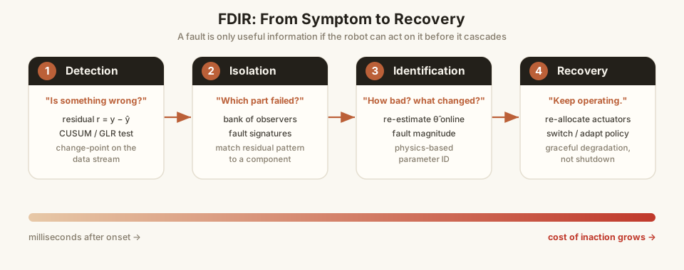
Figure 2 — A fault is only useful information if the robot can act on it before it cascades.
Isolation typically runs a bank of observers, each tuned to a hypothesis "actuator has failed." The residual that stays small tells you which hypothesis is true — a structured-residual or generalized-likelihood-ratio (GLR) test:
The change-detection results above generalize this idea from "did a change happen" to "which of several unknown changes happened," which is precisely the isolation problem. Once isolated, the robot must do two things at once: reconfigure what it controls with (Section 3) and re-identify its now-altered physics (Section 4).
3. Reorienting the Survivors: Control Reconfiguration
Suppose isolation reports: tendon #3 has snapped. A rigid 6-DOF arm with a dead joint is often simply broken. A high-DOF, redundant robot — a humanoid, a multi-tendon tentacle — has a priceless property: there is usually more than one way to produce the motion it needs. Recovery is then a control-allocation problem.
Let be the actuator commands and the desired task wrench (force/torque), related by the actuation matrix :
The minimum-effort command is the pseudo-inverse solution . When tendon fails, we simply delete its column, , and re-solve. The task is still achievable iff lies inside the attainable set of the surviving actuators (the image of the command box under ). Redundancy literally is the safety margin — and it is a gift of high dimensionality.
Loading Interactive Python Environment...
The required force still sits comfortably inside the shrunken (dashed) polygon, and the surviving tendons stay within their limits — so the robot keeps working, just with less margin. The deeper challenge is that right after a fault, the model used to compute is wrong (the dynamics just changed), so the controller must remain stable despite model error.
🔬 Research Spotlight — Robustness to Modeling Errors in Risk-Sensitive Markov Decision Problems (arXiv:2209.12937)
Contribution: policies for risk-sensitive MDPs that come with explicit guarantees on how performance degrades when the model is wrong, using Markov risk measures.
Why it matters for deployment: reconfiguration happens at the worst possible moment — the instant your model became inaccurate. A risk-sensitive, robustly-designed controller degrades gracefully under that mismatch instead of going unstable, which is the difference between a limp-home mode and a crash.
4. Parameter Identification with Physical Models
Reconfiguration buys time; the robot then has to learn its new body. Rather than discarding physics for a black-box network, deployable systems use gray-box identification: keep the physical structure, fit only the parameters that changed. Recall the key fact from Part 4 — rigid-body dynamics are linear in the inertial parameters:
where is the (known) regressor and stacks masses, inertias, friction, and tendon-stretch coefficients. Linearity means we can identify online with Recursive Least Squares (RLS):
Loading Interactive Python Environment...
The estimate locks onto the true parameters within a couple hundred noisy measurements — provided the trajectory is persistently exciting. But does such a recursive, noise-driven estimator always converge, and to what? That guarantee is not obvious, and it is the subject of foundational work from the lab.
🔬 Research Spotlight — Convergence of Recursive Stochastic Algorithms using Wasserstein Divergence (arXiv:2003.11403) and Probabilistic Contraction Analysis of Iterated Random Operators (arXiv:1804.01195)
Contribution: general conditions under which recursive stochastic algorithms (the family that includes RLS, stochastic gradient, and adaptive filters) converge, analyzed through Wasserstein-divergence contraction and the theory of iterated random operators.
Why it matters for deployment: online parameter ID is a recursive stochastic algorithm running on noisy data. These results say when the estimator is guaranteed to settle to the true physics rather than wander or diverge — the mathematical license to trust a self-identifying robot in the field.
5. The Role of Sensing
Every block so far — residuals, isolation, allocation, identification — consumes an estimate of the state . Sensing is the foundation the whole loop stands on. Two ideas govern it:
- Observability. Can the internal state even be reconstructed from the available measurements? Formally, the observability Gramian must be full-rank. For a high-DOF continuum robot this is delicate: you have far more states than sensors, so clever proprioception (embedded strain gauges, fiber-Bragg-grating shape sensing, vision) is what keeps the system observable at all.
- Fusion. Real estimates come from an Extended Kalman Filter or a particle filter blending a physics model with noisy, asynchronous sensors:
The danger: an estimator is only as trustworthy as its sensors. A spoofed measurement quietly corrupts , and every downstream block — detection, control, learning — inherits the lie. Hardening the observer itself against tampering closes that gap.
🔬 Research Spotlight — Adversarial Reinforcement Learning for Observer Design in Autonomous Systems under Cyber Attacks (arXiv:1809.06784)
Contribution: a state observer trained adversarially — against a worst-case attacker — so that estimation stays accurate even when sensor channels are actively compromised.
Why it matters for deployment: it fuses the two themes of this post. Sensing underpins everything, and security threats target sensing first. An observer designed to survive a strategic attacker protects the entire fault-tolerant loop at its most vulnerable point.
For a deeper, lecture-style treatment of the stochastic-control and estimation machinery behind this section, see Prof. Gupta's lecture series on YouTube.
6. Multi-Task Reinforcement Learning for New Tasks
A deployed robot is rarely asked to do one thing forever. New tasks arrive: a new object to grasp, a new gap to squeeze through. Re-training from scratch each time is hopeless on hardware. The answer is multi-task RL: train one task-conditioned policy , where the context names the task, sharing structure across tasks so the next one is cheap:
The payoff is transfer: a new task warm-started from the shared policy starts far up the learning curve instead of at zero.
Loading Interactive Python Environment...
Two realities make this hard on a physical robot: the cost signal is often unbounded (energy, large failure penalties), which breaks much of standard RL theory; and you usually cannot explore freely on hardware, so you must learn from logged data and deploy under a tight compute budget (the edge constraints of Part 8).
🔬 Research Spotlight — Operator-Theoretic Foundations and Policy Gradient Methods for General MDPs with Unbounded Costs (arXiv:2603.17875)
Contribution: rigorous operator-theoretic foundations and convergent policy-gradient methods for general MDPs with unbounded costs — the regime most real robotic objectives actually live in.
Why it matters for deployment: energy budgets and catastrophic-failure penalties are unbounded. A learning method proven to converge under those costs is what lets you trust an RL controller on expensive hardware instead of hoping it behaves.
🔬 Research Spotlight — Offline RL With Resource Constrained Online Deployment (arXiv:2110.03165)
Contribution: a framework that learns policies offline from logged experience while explicitly respecting the limited compute available at deployment.
Why it matters for deployment: a field robot cannot run millions of risky trials, and its onboard processor is small. Learning offline and deploying cheaply is the only practical route to adding new skills after the robot has left the lab.
A companion to this — and a recurring lecture topic — is the foundational theory of reinforcement learning and approximate dynamic programming; Prof. Gupta's YouTube lectures work through the stochastic-control roots of these methods.
7. Cybersecurity: The Adversary in the Loop
Every channel in Figure 1 that carries data or commands is also a channel an adversary can exploit. A robot on a network is a cyber-physical system, and a clever attacker need not break it physically — corrupting its information is enough.
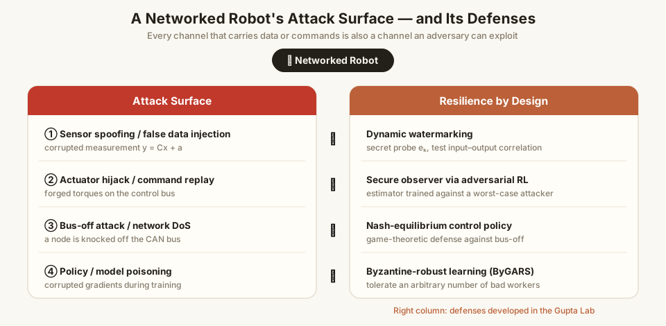
Figure 3 — Each threat (left) has a principled defense (right). The defenses shown were developed in the Gupta Lab.
The most insidious attack is false data injection: the measurement becomes , with crafted to slip past the residual test of Section 1. You cannot detect it by watching outputs alone — so you make the inputs unpredictable to the attacker.
🔬 Research Spotlight — A Dynamic Watermarking Algorithm for Finite Markov Decision Problems (arXiv:2111.04952)
Contribution: a dynamic watermarking scheme that superimposes a secret, private random signal on the control input and then statistically tests whether the measured response carries the expected watermark.
Why it matters for deployment: if a sensor stream has been faked, it will not correlate with the secret probe, and the tamper is exposed — even when the false data was specifically designed to fool a passive detector. This is active integrity for the sensing channel.
At the network layer, robots run on buses like CAN, where a bus-off attack can knock a node offline — a targeted denial of service. Defending it is naturally a game between attacker and controller.
🔬 Research Spotlight — Nash Equilibrium Control Policy against Bus-off Attacks in CAN Networks (arXiv:2111.04950)
Contribution: a game-theoretic (Nash-equilibrium) control policy that keeps a node alive on the CAN bus under bus-off attacks.
Why it matters for deployment: the communication fabric every multi-actuator robot relies on is a real attack surface. Treating defense as an equilibrium strategy against a strategic adversary yields guarantees a fixed heuristic cannot.
Finally, when a fleet of robots learns collaboratively, the threat moves to training time: a few compromised units can poison the shared model with corrupted gradients.
🔬 Research Spotlight — ByGARS: Byzantine SGD with Arbitrary Number of Attackers (arXiv:2006.13421)
Contribution: robust distributed training that tolerates an arbitrary number of Byzantine (malicious) workers by learning server-side reputation weights for each contributor.
Why it matters for deployment: fleet learning and federated updates are how a robot population improves. ByGARS keeps that pipeline trustworthy even when an unknown fraction of the fleet is adversarial.
High-Dimensional vs. Low-Dimensional: Resilience, Restated
The series' recurring theme returns one last time — and here, for once, high dimensionality helps as often as it hurts.
| Aspect | Low-dim (6-DOF arm) | High-dim (continuum octopus) |
|---|---|---|
| Fault tolerance | A dead joint often halts the task | Redundancy lets surviving actuators take over (Section 3) |
| Detection | Few residual channels; easy to monitor | Many correlated channels; needs model-free, mixing-aware detectors |
| Parameter ID | Handful of parameters | interacting parameters that drift continuously (Part 5) |
| Sensing | A few encoders suffice | Observability is fragile; proprioception is essential (Section 5) |
| Attack surface | Few nodes, simple bus | Many nodes, rich network — larger surface to defend (Section 7) |
| Net effect | Simpler to secure, brittle to faults | Harder to secure, but gracefully degradable |
Redundancy is the double edge: it is the very thing that lets a high-DOF robot survive a broken actuator, and the thing that makes its dynamics, sensing, and security so much harder to pin down.
Focus on the Octopus: A Body That Heals Itself
For our metallic continuum octopus, this loop is not optional — it is the product. A tentacle has dozens of tendons; over a long mission some will stretch, fray, or snap, and some sensor will drift. The octopus is designed to treat that as a Tuesday:
- Detect the anomaly in the proprioceptive stream the instant a tendon's behavior shifts (Section 1).
- Isolate the failed tendon via a bank of observers (Section 2).
- Reconfigure — re-solve the tendon allocation so the remaining tendons reproduce the commanded curvature (Section 3); a high-DOF tentacle almost always has a spare way to bend.
- Re-identify the changed stretch and friction coefficients online, keeping the model honest (Section 4, building on the recalibration story of Part 5).
- Re-learn any genuinely new task by transfer from the shared multi-task policy (Section 6).
- Defend every sensor and bus carrying these signals against tampering (Section 7).
A robot that does all six is no longer a fragile lab demonstration. It is a system you can deploy — which is where the science stops being a paper and starts being a machine in the world. That is the goal of the whole series, and a fitting place to end.
Thanks for reading "Robotics Zero to Hero." From the geometry of a single rotation in Part 1 to a self-healing, secure, learning robot here in Part 10 — the throughline has always been the same: the tools that feel effortless in low dimensions are exactly the ones we must reinvent to make high-dimensional, real-world robots survive.
The Research Behind This Post
The contributions highlighted above come from the lab of Prof. Abhishek Gupta (Department of Electrical and Computer Engineering, The Ohio State University; founder of Ensemble Control). Explore the full body of work:
- arXiv (all papers): arxiv.org/a/gupta_a_1
- Personal website & publications: gupta706.github.io
- Lectures on YouTube (reinforcement learning, stochastic control, optimization): youtube.com/@abhigup
Papers cited, by theme
Anomaly & change detection
- Model-Free Change Point Detection for Mixing Processes — arXiv:2312.09197
- Change Detection of Markov Kernels with Unknown Pre and Post Change Kernel — arXiv:2201.11722
- Hoeffding's Inequality for Markov Chains under Generalized Concentrability Condition — arXiv:2310.02941
Identification & convergence of recursive estimators
- Convergence of Recursive Stochastic Algorithms using Wasserstein Divergence — arXiv:2003.11403
- Probabilistic Contraction Analysis of Iterated Random Operators — arXiv:1804.01195
Reinforcement learning, robustness & deployment
- Operator-Theoretic Foundations and Policy Gradient Methods for General MDPs with Unbounded Costs — arXiv:2603.17875
- Offline RL With Resource Constrained Online Deployment — arXiv:2110.03165
- Robustness to Modeling Errors in Risk-Sensitive Markov Decision Problems with Markov Risk Measures — arXiv:2209.12937
Sensing & cybersecurity of cyber-physical systems
- Adversarial Reinforcement Learning for Observer Design in Autonomous Systems under Cyber Attacks — arXiv:1809.06784
- A Dynamic Watermarking Algorithm for Finite Markov Decision Problems — arXiv:2111.04952
- Nash Equilibrium Control Policy against Bus-off Attacks in CAN Networks — arXiv:2111.04950
- ByGARS: Byzantine SGD with Arbitrary Number of Attackers — arXiv:2006.13421
Further reading: Basseville & Nikiforov, "Detection of Abrupt Changes" (1993) for CUSUM/GLR; Blanke et al., "Diagnosis and Fault-Tolerant Control" (2016) for FDIR; Ljung, "System Identification" (1999) for recursive estimation; Cardenas et al. on secure control of cyber-physical systems.
Interested in the research?
We collaborate with researchers, engineers, and institutions pushing Physical AI into extreme environments. Get in touch to explore working with the lab.
Collaborate with us